Building an AI Radio Scanner for $220: RTL-SDR Meets Machine Learning
How I built an automatic radio signal classifier using an ARM single-board computer and machine learning, with spectrograms to prove it works
If you have spent any time scanning the RF spectrum with an RTL-SDR, you know the drill. Tune to a frequency, see activity on the waterfall, Google the frequency, try different demodulation modes, still not sure what you are hearing, and repeat 500 times.
After digging through r/RTLSDR and r/amateurradio, I found threads going back nearly a decade asking if anyone had used neural networks for automatic signal recognition. The answers were always the same: academic papers with synthetic data, expensive GPU setups, or "sounds cool but no tutorial."
The RTL-SDR community needed something practical: real-world signals, affordable hardware under $300, and complete code from capture to classification with reproducible results. So I built it.
📁Get the Code
Repository: github.com/TrevTron/rtl-ml
Dataset: HuggingFace
The Hardware: $220 All-In
Indiedroid Nova ($179.95)
The Nova uses the RK3588S processor with a 6 TOPS NPU and 16GB RAM running Debian 12. It is ARM64 architecture, similar to a Raspberry Pi but with dedicated AI hardware. Perfect for edge ML without cloud dependencies.
RTL-SDR Blog V4 ($39.95)
The V4 uses the Rafael Micro R828D tuner covering 500 kHz to 1.7 GHz with 1 PPM TCXO stability and a built-in HF upconverter. Important: the V4 requires the rtl-sdr-blog fork driver, not the default kernel driver. The R828D tuner made a noticeable difference in signal quality during capture compared to generic dongles I tested previously.
Total: $219.90 compared to $2000+ for a GPU workstation and professional SDR.
Raspberry Pi 5 Compatibility
I also tested the entire pipeline on a Raspberry Pi 5. The same code runs on both platforms with no modifications and achieves the same 96.9% accuracy.
| Metric | Indiedroid Nova | Raspberry Pi 5 |
|---|---|---|
| Processing Time | ~102ms | 122ms |
| Feature Extraction | ~90ms | 108ms |
| Model Inference | ~12ms | 14ms |
| Accuracy | 96.9% | 96.9% |
The Pi 5 is about 20% slower but both are real-time capable since 122ms is well under the 500ms capture window.
💡Key Insight
For most users the Pi 5 is the better choice given its availability and community support. The Nova is worth it if you plan to use the NPU for future projects.
The Signals: 7 Types, Decoder-Validated
I built the classifier around 7 signal types that the SDR community actually uses:
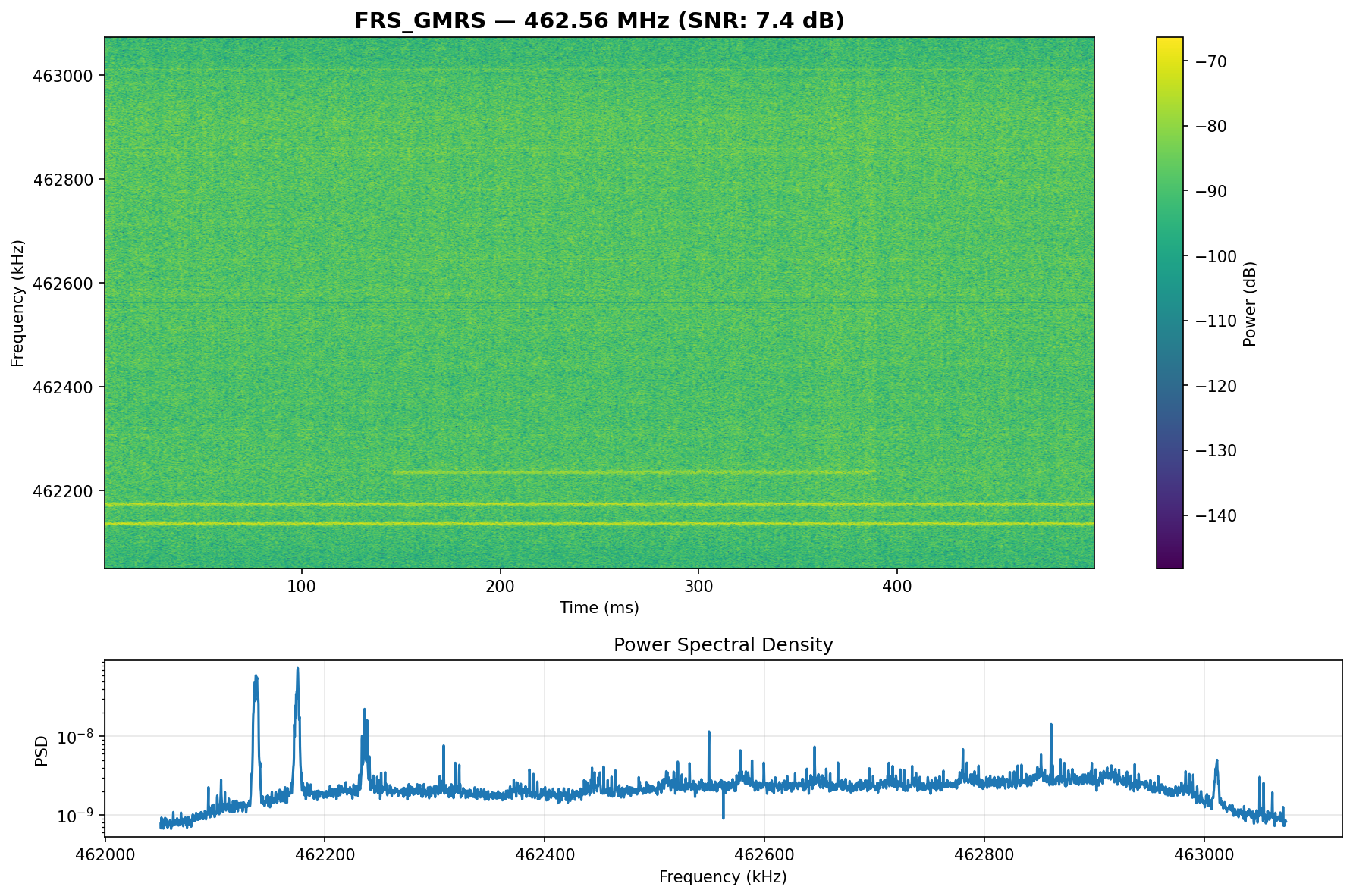
FRS/GMRS (462.5625 MHz)
Family and general mobile radio. Short bursty transmissions.
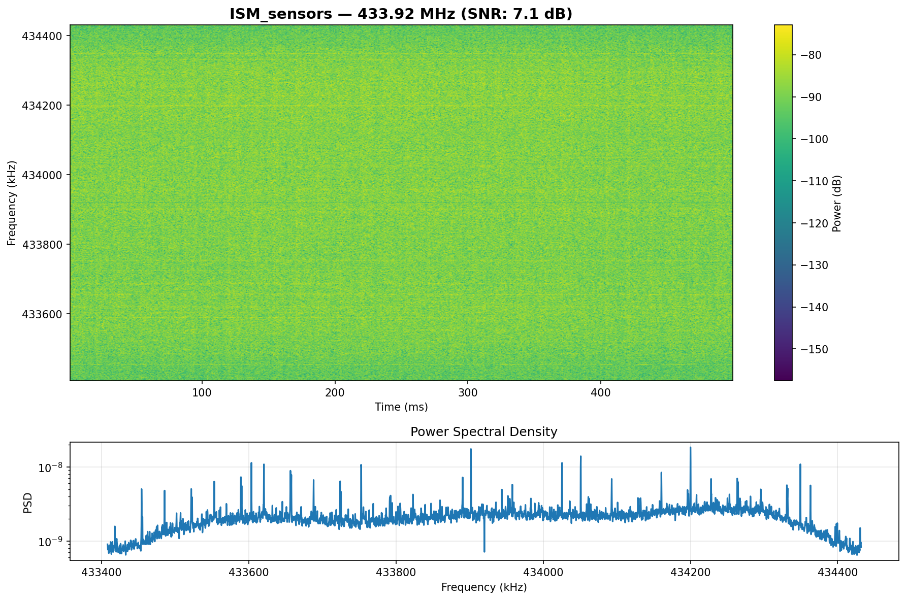
ISM Sensors (433.92 MHz)
Wireless sensors. 20.6x burst ratio.
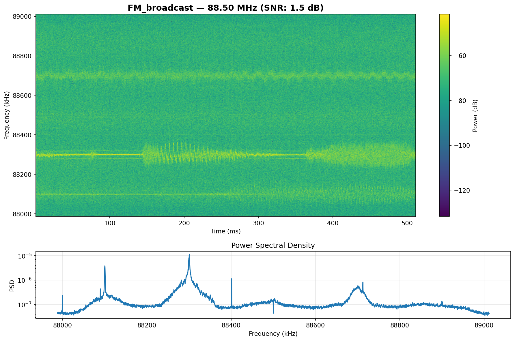
FM Broadcast (88.5–105.7 MHz)
Commercial radio from 5 frequencies. 200 samples for generalization.
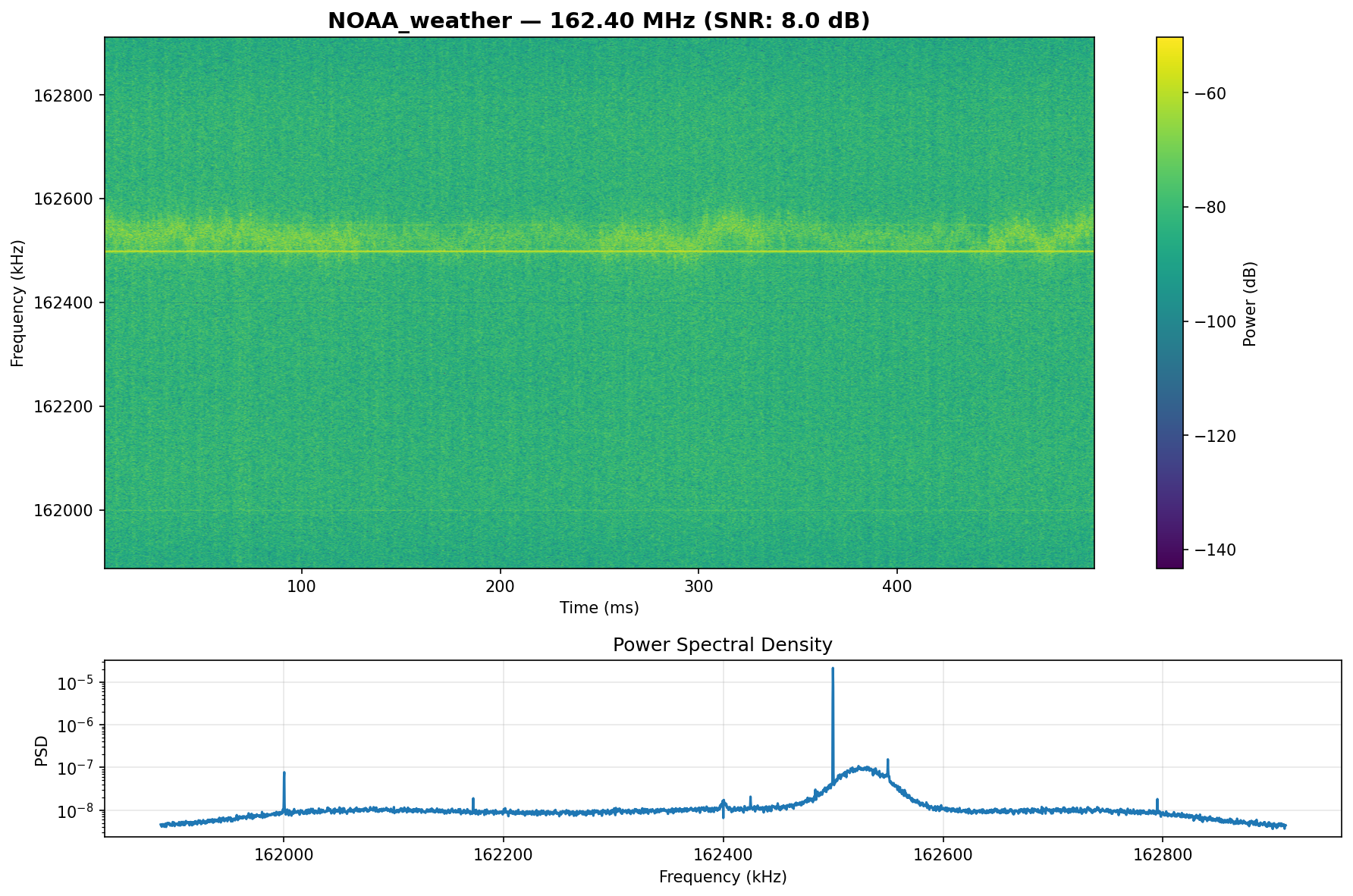
NOAA Weather (162.4 MHz)
Emergency alerts. 14.4 dB SNR.
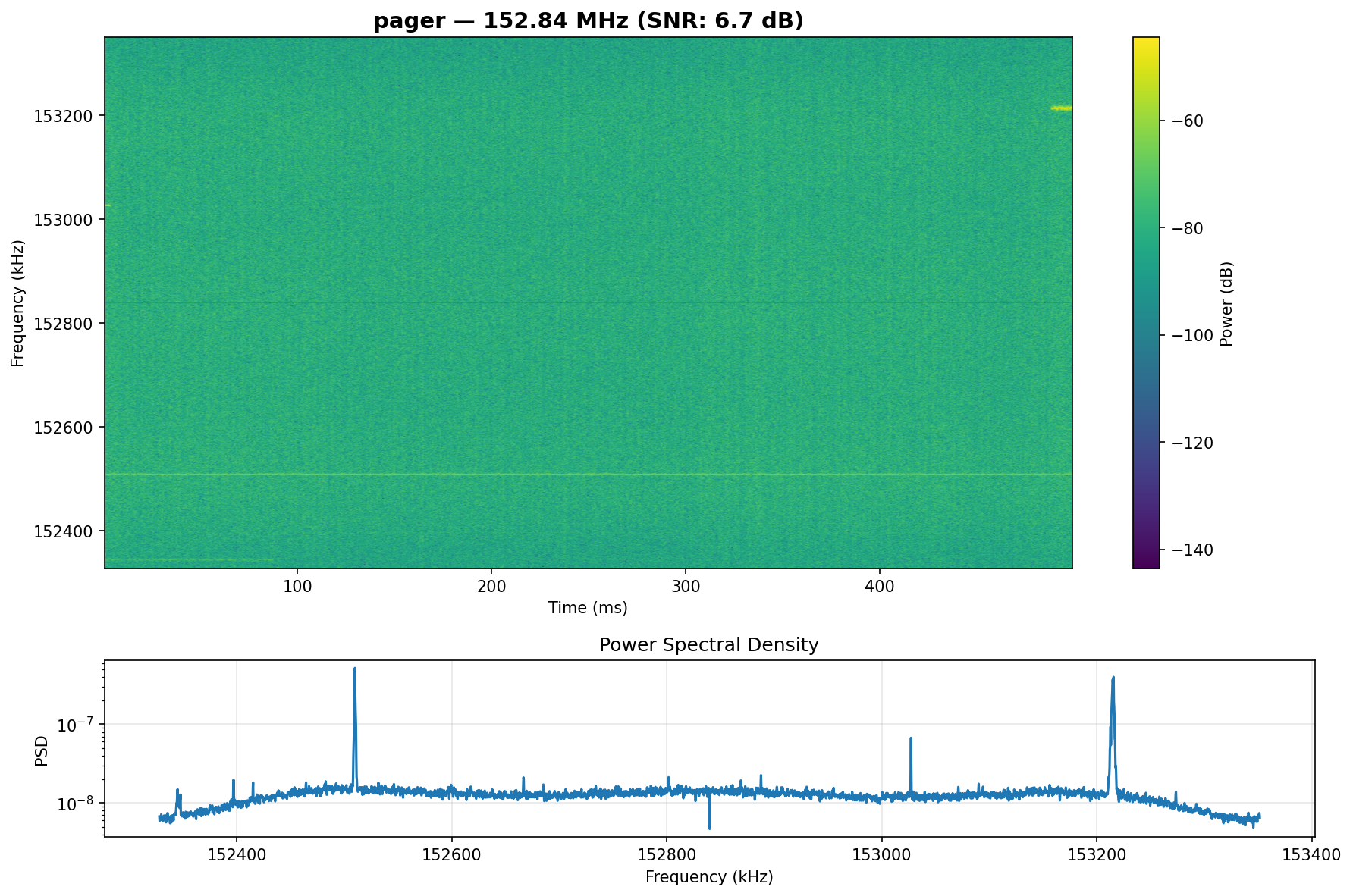
Pager (152.84 MHz)
POCSAG networks. Validated with multimon-ng.
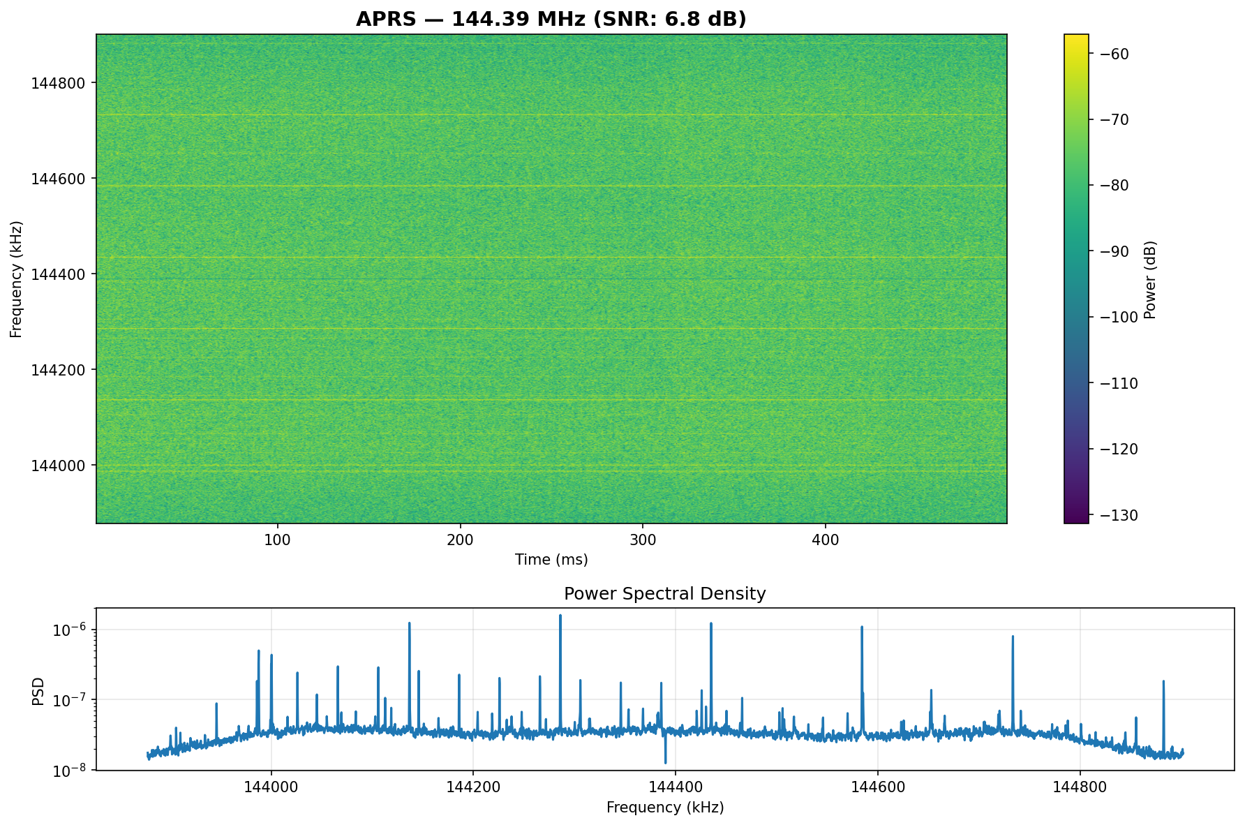
APRS (144.39 MHz)
Ham radio packets. Sparse bursts at 12.7 dB SNR.
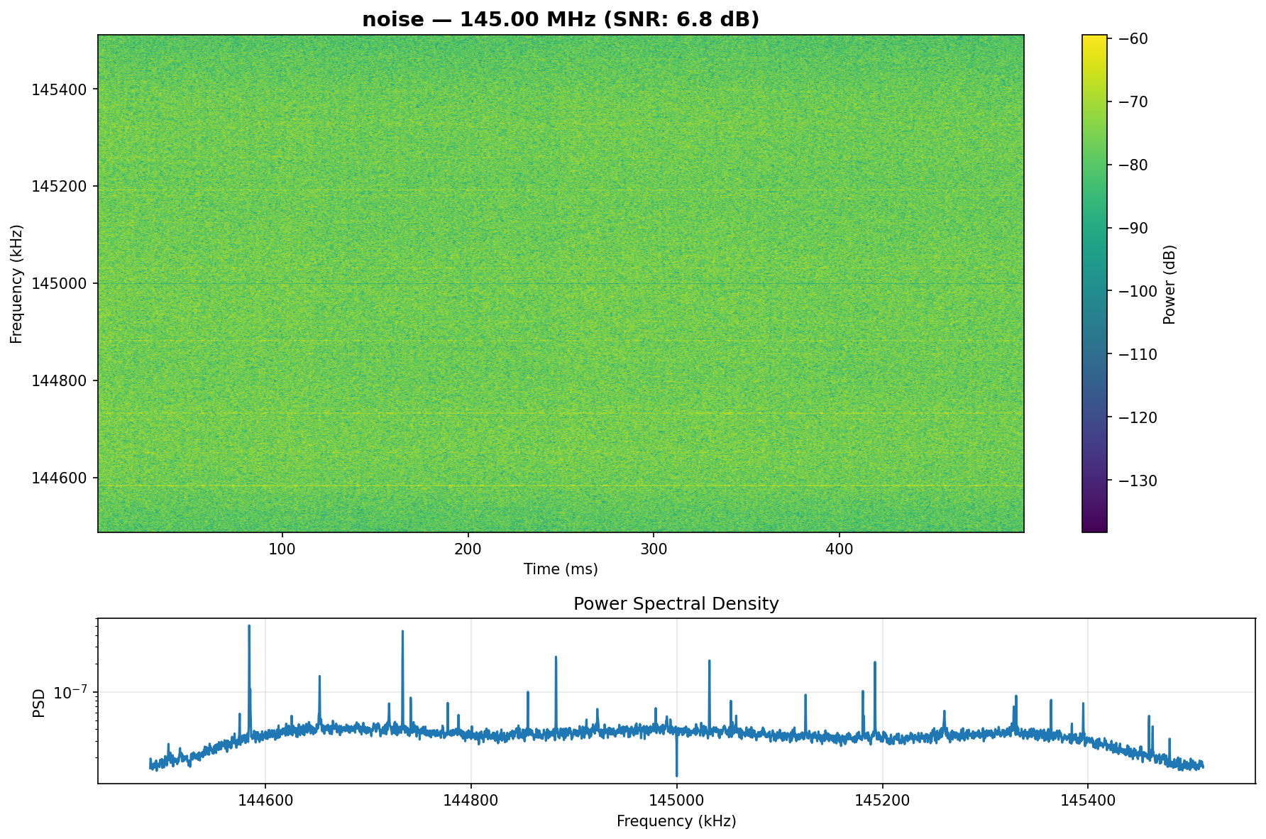
Noise (145 MHz)
Baseline noise floor reference.
Every signal was validated using established decoders to ensure the dataset was grounded in reality, not simulations.
The Dataset: 800 Validated Samples
The capture process was straightforward. For each signal type, I tuned to the frequency, captured 100 samples at 0.5 seconds each (200 for FM broadcast across 5 frequencies), generated spectrograms for visual proof, validated with decoder tools, and saved as .npy files with metadata.
Results:
- • 800 total samples (7 classes, 100–200 per class)
- • 6.5GB dataset
- • 7 spectrograms for visual validation
- • Validation report proving signals are real
Key validation findings:
- ISM sensors: 20.6x burst ratio showing sporadic transmissions
- NOAA weather: 14.4 dB SNR showing strong continuous signal
- Pager and APRS: 12.7 dB SNR showing packet-based transmissions
- FRS/GMRS: Short bursty transmissions on 462.5625 MHz
The dataset is available on Hugging Face so you can reproduce the entire workflow.
The Machine Learning: 17 Features + Random Forest
Every 0.5-second signal sample gets reduced to 17 numerical features covering power statistics, frequency domain characteristics, I/Q analysis, phase behavior, and bandwidth.
Feature Extraction
pythondef extract_features(self, samples):
"""Extract 17 features from IQ samples."""
features = []
# Power calculations
power = np.abs(samples) ** 2
features.append(np.mean(power))
features.append(np.std(power))
features.append(np.max(power))
features.append(np.min(power))
# FFT analysis
fft_vals = np.fft.fft(samples)
fft_power = np.abs(fft_vals) ** 2
features.append(np.mean(fft_power))Full 17-feature extraction available in the repository.
I tested three algorithms:
- Random Forest: 96.9% accuracy (winner)
- SVM: 64.6% accuracy
- K-NN: 77.1% accuracy
Random Forest won because it handles non-linear relationships well, resists overfitting with 100 trees voting, delivers fast inference under 100ms per sample, and produces a tiny 186KB model that fits comfortably on ARM hardware.
Why Feature Extraction Instead of Neural Networks?
I went with feature extraction and Random Forest instead of feeding raw IQ samples into a neural network for a few reasons:
- 240 samples was enough for v1 and 800 samples trains effectively for v2. Neural networks typically need thousands to millions of samples to generalize well.
- The model is 186KB and runs inference in under 15ms on ARM hardware without a GPU.
- The 17 features are interpretable so you can see exactly what the model uses to distinguish signals.
Raw IQ neural networks make more sense when you have large labeled datasets, GPU compute available, and need to classify subtle modulation differences that handcrafted features might miss. For hobbyist-accessible edge deployment on a Pi or similar SBC, feature extraction wins on practicality.
The Results: 96.9% Accuracy
The system achieved perfect 100% classification for five signal types:
- • FM broadcast (40/40 correct)
- • NOAA weather (20/20 correct)
- • APRS (20/20 correct)
- • Noise (20/20 correct)
- • ISM sensors (20/20 correct)
The remaining confusion: 3 FRS/GMRS samples misclassified as ISM sensors (similar bursty patterns), and 2 pager samples misclassified as APRS (similar packet-based transmissions).
Confusion Matrix:
              FM  NOAA_w  APRS  Noise  ISM  FRS  Pager
FM_broadcast  40     0      0      0    0    0     0
NOAA_weather   0    20      0      0    0    0     0
APRS           0     0     20      0    0    0     0
Noise          0     0      0     20    0    0     0
ISM_sensors    0     0      0      0   20    0     0
FRS_GMRS       0     0      0      0    3   17     0
Pager          0     0      2      0    0    0    18
Real machine learning means real confusion. That is expected when working with actual RF data instead of synthetic waveforms.
ℹ️Why FRS/GMRS vs ISM Confusion?
FRS/GMRS and ISM sensors both use short bursty transmissions at UHF frequencies. Their power envelopes overlap significantly, which makes frequency-domain features alone insufficient for perfect separation. Additional time-domain analysis could help distinguish the modulation patterns.
The Implementation: Three Steps
The workflow breaks down into capture, train, and classify.
Step 1: Capture
Signal Capture
pythondef capture_signal(self, frequency, duration=0.5):
self.sdr.center_freq = frequency
time.sleep(0.1) # Settle time for PLL lock
num_samples = int(self.sdr.sample_rate * duration)
samples = self.sdr.read_samples(num_samples)
samples = samples - np.mean(samples) # DC offset removal
time.sleep(0.2)
return samplesStep 2: Train
Training
pythonfrom sklearn.ensemble import RandomForestClassifier
from sklearn.preprocessing import StandardScaler
# Load 800 samples, extract 17 features each
X, y, timestamps = load_dataset('datasets_validated/')
# Temporal split: train on earlier captures, test on later
split_idx = int(len(X) * 0.8)
X_train, X_test = X[:split_idx], X[split_idx:]
y_train, y_test = y[:split_idx], y[split_idx:]
# Normalize features
scaler = StandardScaler()
X_train_scaled = scaler.fit_transform(X_train)
X_test_scaled = scaler.transform(X_test)
# Train Random Forest
model = RandomForestClassifier(n_estimators=100)
model.fit(X_train_scaled, y_train)
# Test: 96.9% accuracy (155/160 correct)
print(f"Accuracy: {model.score(X_test_scaled, y_test):.1%}")Step 3: Classify
Classification
pythondef classify_signal(sdr, model, scaler, class_names, frequency, duration=0.5):
"""Capture and classify a signal"""
sdr.center_freq = frequency
time.sleep(0.1)
samples = sdr.read_samples(int(sdr.sample_rate * duration))
samples = samples - np.mean(samples) # DC offset removal
features = extract_features(samples)
features_scaled = scaler.transform([features])
prediction = model.predict(features_scaled)[0]
class_name = class_names[prediction]
return class_nameFull classification logic with probabilities available in the repository.
The complete code is available in the GitHub repository with setup instructions that take about 30 minutes from clone to working classifier.
Why This Matters for the Community
This project addresses a gap that has existed in the RTL-SDR community for years. The hardware exists, the software libraries exist, but there has not been a practical guide that bridges the two using real-world signals and affordable equipment.
For hobbyists, this means you can build an automatic scanner that skips noise and logs interesting signals without manually checking every frequency. For researchers working on spectrum monitoring or IoT security, this provides a low-cost entry point for automated signal intelligence. For educators, this demonstrates how to integrate electrical engineering and data science in a project that students can actually reproduce with accessible hardware.
Building on ARM: Challenges and Solutions
Working with ARM hardware brought specific challenges. Initially, I struggled with USB overflow errors until I optimized the sample rate to 1.024 MSPS. That sample rate is deliberately chosen for ARM processors because it is fast enough for most signals but low enough to avoid saturating the USB bus on single-board computers.
⚠️ARM Gotcha
USB overflow errors are common on ARM SBCs. The 1.024 MSPS sample rate is deliberately chosen - fast enough for most signals but low enough to avoid saturating the USB bus.
Real-world data is messy. A model trained on clean synthetic waveforms will fail the moment you attach a real antenna in a noisy urban environment. I am in a busy Southern California suburb which means I am dealing with interference from broadcast FM, cellular towers, ISM devices, and everything else that shares the spectrum. The validation process using actual decoders like multimon-ng and rtl_433 was critical for ensuring the dataset represented real signals, not idealized simulations.
DC offset from the RTL-SDR tuner was a significant factor in v1 accuracy issues. Version 2.0 added explicit DC removal during capture, which improved feature extraction quality across all signal types. Multi-frequency FM sampling (5 stations instead of 1) also improved generalization by preventing the model from memorizing a single station's characteristics.
What's Next for This Project
With v2.0 complete (96.9% accuracy, 7 signal types, 800 samples), here is what is next:
NPU acceleration is the obvious next step. The Nova's 6 TOPS AI chip is currently unused. Offloading inference to the NPU would enable multi-channel real-time classification across the entire bandwidth instead of single-frequency sequential scanning.
A web dashboard for browser-based monitoring would make the system more accessible. Instead of SSH'ing into the Nova to check results, you would have a real-time display showing classified signals as they are detected.
More signal types would expand the use cases. Adding modes like SSB, CW, LoRa, and digital voice modes (DMR, D-STAR) would make the classifier more practical for ham radio operators and researchers working with a wider range of protocols.
RF fingerprinting is another potential direction. The current 17 features target signal type classification. For device fingerprinting you would need features that capture hardware traits like carrier frequency offset, phase noise characteristics, and I/Q imbalance. The capture, extract, classify architecture would work the same way but the feature extraction would focus on hardware signatures rather than modulation characteristics.
If you have ideas or want to contribute, the repository is open for pull requests.
Try It Yourself
Requirements:
- • Indiedroid Nova, Raspberry Pi 4/5, or Orange Pi 5
- • RTL-SDR Blog V4 (or V3)
- • Antenna (dipole, discone, or wire)
- • 30 minutes for setup
Quick Start
bashgit clone https://github.com/TrevTron/rtl-ml
cd rtl-ml
pip install -r requirements.txt
# Capture your own data (optional)
python3 capture_validated.py
# Train model (optional - pre-trained included)
python3 train_validated.py
# Classify live signals
python3 classify_live.py --freq 98.7e6Expected time: 30 minutes to working classifier using the pre-trained model, or 1 hour if capturing your own dataset.
Acknowledgments
Hardware:
RTL-SDR Blog V4 provided by RTL-SDR Blog.
Community Input:
- • r/RTLSDR - Feature requests and signal suggestions
- • r/amateurradio - Ham radio expertise
- • r/sdr - Technical validation
Open Source Tools:
- • pyrtlsdr - RTL-SDR Python bindings
- • scikit-learn - ML framework
- • matplotlib / scipy - Visualization
Bottom Line
You do not need a PhD, expensive hardware, or cloud compute to build an AI-powered radio signal classifier. With $220 of hardware, Python, and real-world signal captures, you can build a system that automatically identifies FM broadcasts, weather radio, pager networks, ISM sensors, and more with 96.9% accuracy.
The model runs entirely on ARM hardware without cloud dependencies. The inference takes under a second. The setup process takes under an hour. The results are validated with spectrograms and decoder tools so you can verify everything yourself.
What will you classify next?
Repository: github.com/TrevTron/rtl-ml
Dataset: HuggingFace dataset
Author: Trevor Unland | AI Systems Builder and Technical Researcher
Contact: unland.dev | LinkedIn
Hardware provided by RTL-SDR Blog.
All code released under MIT license.
Get notified when I publish new hardware reviews, benchmarks, and security research. No spam, unsubscribe anytime.
I respect your privacy. Powered by Buttondown.